Convergence of Sequences (1)

Pablo Winant

Life of a computational economist

We spend a lot of time waiting for algorithms to converge!
- solution 1: program better
- solution 2: better algorithms
- even better: understand convergence properties (information about the model)

Recursive sequence

Consider a function \(f: \mathbb{R}^n\rightarrow \mathbb{R}^n\) and a recursive sequence \((x_n)\) defined by \(x_0\in \mathbb{R}^n\) and \(x_n = f(x_{n-1})\).

We want to compute a fixed point of \(f\) and study its properties.

Today: Some methods for the case \(n=1\).

Another day:

the matrix case: \(x_n = A^n x_0\) where \(A\in \mathbb{R}^{n\times n}\)
the finite nonlinear case: \(x_n = f(x_{n-1})\)

Example: growth model

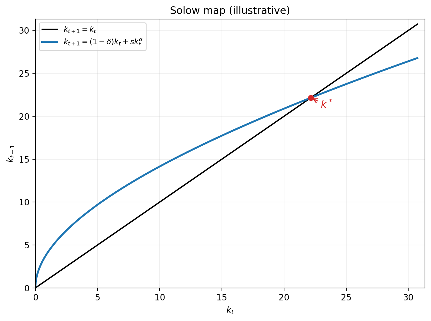
Solow growth model:

capital accumulation	\(k_t = (1-\delta)k_{t-1} + i_{t-1}\)
production	\(y_t = k_t^\alpha\)
consumption	\(c_t = (1-{\color{red}s})y_t\)
investment	\(i_t = s y_t\)

For a given value of \({\color{red} s}\in\mathbb{R}^{+}\) ( \({\color{red} s}\) is a decision rule) \[k_{t+1} = f(k_t, {\color{red} s})\]

backward-looking iterations
Solow hypothesis: saving rate is invariant

Questions:

What is the steady-state?
Can we characterize the transition back the steady-state?
Characterize the dynamics close to the steady-state?
what is the optimal \(s\) ?

Another example: linear new keynesian model

Basic New Keynesian model (full derivation if curious )

new Phillips curve (PC):\[\pi_t = \beta \mathbb{E}_t \pi_{t+1} + \kappa y_t\]
dynamic investment-saving equation (IS):\[y_t = \beta \mathbb{E}_t y_{t+1} - \frac{1}{\sigma}(i_t - \mathbb{E}_t(\pi_{t+1}) ) - {\color{green} z_t}\]
interest rate setting (taylor rule): \[i_t = \alpha_{\pi} \pi_t + \alpha_{y} y_t\]
persistent shock: \(z_t = \rho z_{t-1} + \varepsilon_t\) ::::: {.fragment}

Solving the system: \(\begin{bmatrix}\pi_t \\\\ y_t \end{bmatrix} = {\color{red} c} z_t\)

The system is forward looking:

take \(\begin{bmatrix}\pi_{t+1} \\\\ y_{t+1} \end{bmatrix} = {\color{red} {c_n}} z_{t+1}\) → deduce \(\begin{bmatrix}\pi_{t} \\\\ y_{t} \end{bmatrix} = {\color{red} {c_{n+1}}} z_{t}\)

\(\mathcal{T}: \underbrace{c_{n}}_{t+1: \; \text{tomorrow}} \rightarrow \underbrace{c_{n+1}}_{t: \text{today}}\) is the time-iteration operator (a.k.a. Coleman operator)

Questions:

What is the limit to \(c_{t+1} = \mathcal{T} c_n\)?
Under which conditions (on \(\alpha_{\pi}, \alpha_y\)) is it convergent?
- determinacy conditions
- interpretation: does the central bank manage to control inflation expectations?

:::

Recursive sequence (2)

🤔 Wait: does a fixed point exist?

we’re not very concerned by the existence problem here
we’ll be happy with local conditions (existence, uniqueness) around a solution

In theoretical work, there are many fixed-point theorems to choose from.

For example:

Brouwer fixed point: assume \(f\) is continuous and there is an interval such that \(f([a,b])\subset[a,b]\). Then we know there exists \(x\) in \([a,b]\) such that \(f(x)=x\). (There can be many such points.)

Example: growth model with multiple fixed points

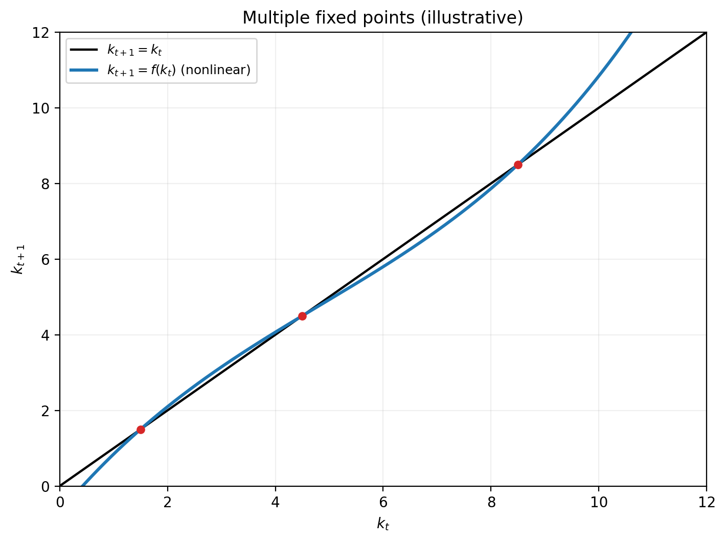
Multiple equilibria in the growth model

In the growth model, if we change the production function: \(y=k^{\alpha}\) for a nonconvex/nonmonotonic one, we can get multiple fixed points.

Convergence

Given \(f: \mathbb{R} \rightarrow \mathbb{R}\) consider the sequence \(x_n = f(x_{n-1})\)

How do we characterize behaviour around \(x\) such that \(f(x)=x\)?

Stability criterion:
- if \(|f^{\prime}(x)|>1\): sequence is unstable and will not converge to \(x\) except by chance
- if \(|f^{\prime}(x)|<1\): \(x\) is a stable fixed point
- if \(|f^{\prime}(x)|=1\): ??? (look at higher order terms, details ↓)

Convergence (Cobweb intuition)

Think of the graph of \(y=f(x)\) and the 45-degree line \(y=x\).

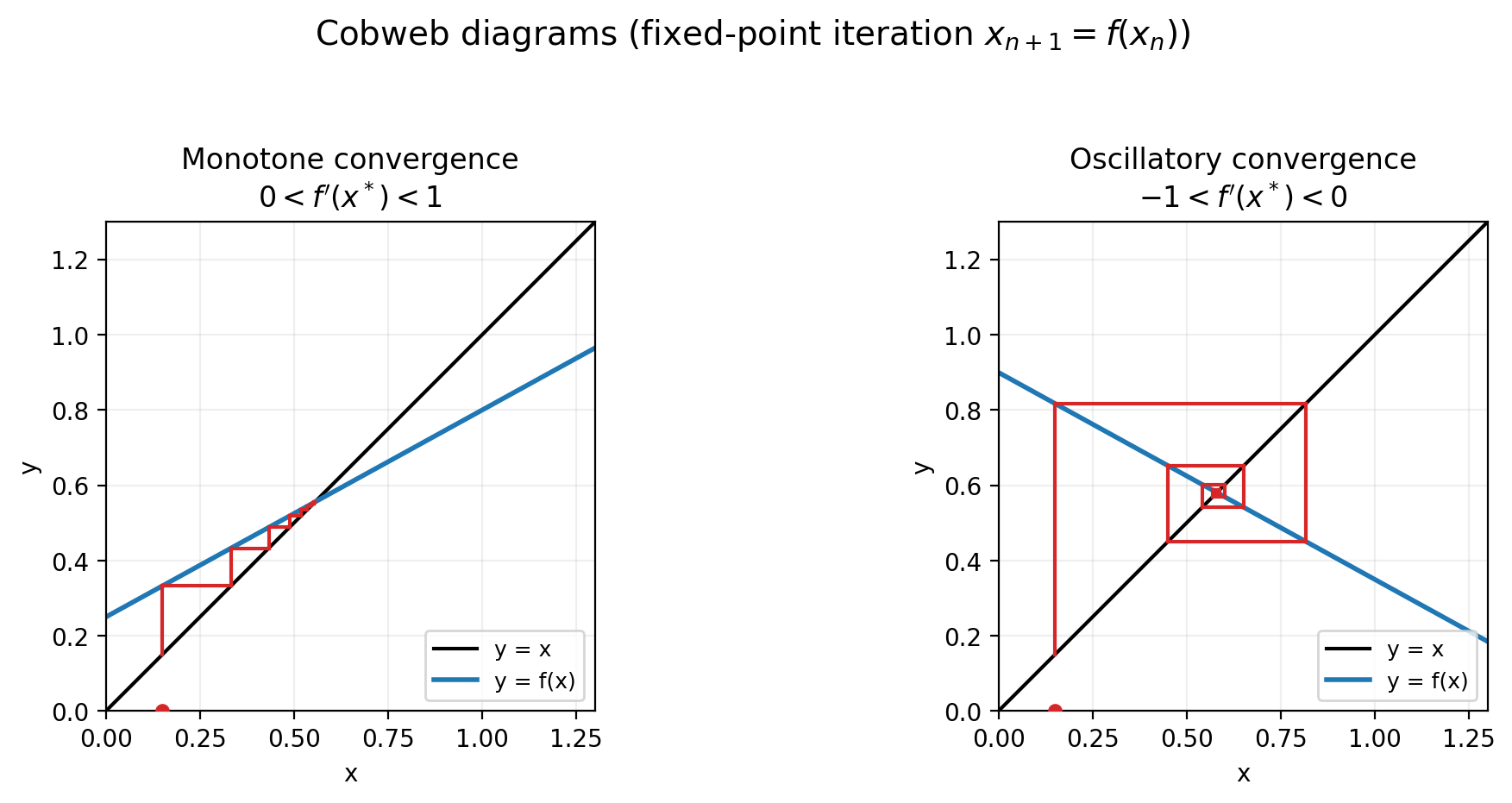
If \(0<f'(x^*)<1\): iterates approach \(x^*\) monotonically.
If \(-1<f'(x^*)<0\): iterates approach \(x^*\) but typically oscillate (alternating sides).
If \(|f'(x^*)|>1\): you generically move away from \(x^*\).

Convergence (first order approximation)

To get the intuition about local convergence, assume you have an initial point \(x_n\) close to the steady state and consider the following expression:

\[x_{n+1} - x = f(x_n) - f(x) = f^{\prime}(x) (x_n-x) + o(x_n-x)\]

If one sets aside the error term (which one can do with full mathematical rigour), the dynamics for very small perturbations are given by:

\[|x_{n+1} - x| \approx |f^{\prime}(x)| |x_n-x|\]

When \(|f^{\prime}(x)|<1\), the distance to the target decreases at each iteration and we have convergence.

When \(|f^{\prime}(x)|>1\) there is local divergence.

This is conform to Cobweb intuition.

Borderline case \(|f'(x^*)|=1\)

When \(|f'(x^*)|=1\), the linear approximation does not tell you whether you converge.

You must look at higher-order terms (Taylor expansion), and behavior can depend on the side you start from.
In practice, treat this as a warning sign: add damping, change the iteration, or switch to a root-finding method.

Change the problem

Sometimes, we are interested in tweaking the convergence speed: \[x_{n+1} = (1-\lambda) x_n + \lambda f(x_n)\]
- \(\lambda\) is the learning rate:
  - \(\lambda>1\): acceleration
  - \(\lambda<1\): dampening

We can also replace the function by another one \(g\) such that \(g(x)=x\iff f(x)=x\), for instance: \[g(x)=x-\frac{f(x)-x}{f^{\prime}(x)-1}\]
- this is the Newton iteration

Contraction mapping (why fixed-point iteration works)

Suppose there exists an interval \(I=[a,b]\) such that \(f(I)\subseteq I\) and \[\sup_{x\in I} |f'(x)| \le L < 1.\]

Then there is a unique fixed point \(x^*\in I\).
For any \(x_0\in I\), iterating \(x_{n+1}=f(x_n)\) converges to \(x^*\).
The error shrinks at least linearly: \(|x_{n+1}-x^*|\le L\,|x_n-x^*|\).

This is the one-dimensional version of the contraction logic used for many “time-iteration” operators in macro.

Dynamics around a stable point

We can write successive approximation errors: \[|x_t - x_{t-1}| = | f(x_{t-1}) - f(x_{t-2})| \] \[|x_t - x_{t-1}| \sim |f^{\prime}(x_{t-1})| |x_{t-1} - x_{t-2}| \]
Ratio of successive approximation errors \[\lambda_t = \frac{ |x_{t} - x_{t-1}| } { |x_{t-1} - x_{t-2}|}\]
When the sequence converges: \[\lambda_t \rightarrow | f^{\prime}(\overline{x}) |\]

Dynamics around a stable point (2)

How do we derive an error bound? Suppose that we have \(\overline{\lambda}>|f^{\prime}(x_k)|\) for all \(k\geq k_0\):

\[|x_t - x| \leq |x_t - x_{t+1}| + |x_{t+1} - x_{t+2}| + |x_{t+2} - x_{t+3}| + ... \]

\[|x_t - x| \leq |x_t - x_{t+1}| + |f(x_{t}) - f(x_{t+1})| + |f(x_{t+1}) - f(x_{t+2})| + ... \]

\[|x_t - x| \leq |x_t - x_{t+1}| + \overline{\lambda} |x_t - x_{t+1}| + \overline{\lambda}^2 |x_t - x_{t+1}| + ... \]

\[|x_t - x| \leq \frac{1} {1-\overline{\lambda}} | x_t - x_{t+1} |\]

How do we improve convergence ?

\[\frac{|x_t - x_{t-1}|} {|x_{t-1} - x_{t-2}|} \sim |f^{\prime}(x_{t-1})| \]

corresponds to the case of linear convergence (kind of slow).

Aitken’s extrapolation

When convergence is geometric, we have: \[ \lim_{t\rightarrow \infty}\frac{ x_{t+1}-x}{x_t-x} = \lambda \in \mathbb{R}^{\star}\]

Which implies:

\[\frac{ x_{t+1}-x}{x_t-x} \sim \frac{ x_{t}-x}{x_{t-1}-x}\]

Aitken’s extrapolation (2)

Take \(x_{t-1}, x_t\) and \(x_{t+1}\) as given and solve for \(x\):

\[x = \frac{x_{t+1}x_{t-1} - x_{t}^2}{x_{t+1}-2x_{t} + x_{t-1}}\]

or after some reordering

\[x = x_{t-1} - \frac{(x_t-x_{t-1})^2}{x_{t+1}-2 x_t + x_{t-1}}\]

Steffensen’s Method:

start with a guess \(x_0\), compute \(x_1=f(x_0)\) and \(x_2=f(x_1)\)
use Aitken’s guess for \(x^{\star}\). If required tolerance is met, stop.
otherwise, set \(x_0 = x^{\star}\) and go back to step 1.

It can be shown that the sequence generated from Steffensen’s method converges quadratically, that is

\(\lim_{t\rightarrow\infty} \frac{x_{t+1}-x_t}{(x_t-x_{t-1})^2} \leq M \in \mathbb{R}^{\star}\)

Convergence speed

Rate of convergence of series \(x_t\) towards \(x^{\star}\) is:

linear: \[{\lim}_{t\rightarrow\infty} \frac{|x_{t+1}-x^{\star}|}{|x_{t}-x^{\star}|} = \mu \in R^+\]
superlinear: \[{\lim}_{t\rightarrow\infty} \frac{|x_{t+1}-x^{\star}|}{|x_{t}-x^{\star}|} = 0\]
quadratic: \[{\lim}_{t\rightarrow\infty} \frac{|x_{t+1}-x^{\star}|}{|x_{t}-x^{\star}|^{\color{red}2}} = \mu \in R^+\]

Convergence speed

Remark: in the case of linear convergence with \(\mu\in(0,1)\),

\[\mu = {\lim}_{t\rightarrow\infty} \frac{|x_{t+1}-x^{\star}|}{|x_{t}-x^{\star}|} = {\lim}_{t\rightarrow\infty} \frac{|x_{t+1}-x_t|}{|x_t-x_{t-1}|}.\]

Moreover, asymptotically one has the useful heuristic bound \[|x_t-x^{\star}| \approx \frac{1}{1-\mu}\,|x_{t+1}-x_t|.\]

Damping / relaxation in practice

Consider the relaxed iteration \[x_{n+1}=g(x_n)=(1-\lambda)x_n+\lambda f(x_n).\]

Locally around a fixed point \(x^*\), \[g'(x^*) = 1-\lambda+\lambda f'(x^*).\]

If you can estimate \(f'(x^*)\approx a\), choose \(\lambda\) to make \(|g'(x^*)|\) small.
The “ideal” choice (unconstrained) is \(\lambda^* = \frac{1}{1-a}\), which gives \(g'(x^*)=0\).
In practice you often restrict \(\lambda\in(0,1]\) (safeguard), so you clamp \(\lambda\) to that range.

In practice

Problem: Suppose one is trying to find \(x\) solving the model \(G(x)=0\)
- An iterative algorithm provides a function \(f\) defining a recursive series \(x_{t+1}\).
The best practice consists in monitoring at the same time:
- the success criterion: \[\epsilon_n = |G(x_n)|\]
  - have you found the solution?
- the successive approximation errors \[\eta_n = |x_{n+1} - x_n|\]
  - are you making progress?
- the ratio of successive approximation errors \[\lambda_n = \frac{\eta_n}{\eta_{n-1}}\]
  - what kind of convergence? (if \(|\lambda_n|<1\): OK, otherwise: ❓)